


Estimate Calibration Accuracy using Residual Error in Calibration Optimizer Flow


We have introduced Calibration Optimiser Flow to calibrate multiple sensors together for high quality calibration resulting in better sensor fusions. In our post explaining the efficacy of the flow, we mention the importance of accurate sensor calibration and the lack of ground truth to assess the calibration results.
In Calibration Optimiser flow, we have introduced a metric called Residual error, which reflects the calibration error of multiple sensors together. Residual error consists of six values each corresponding to the residual of the extrinsic calibration parameters (roll, pitch, yaw, x_position, y_position and z_position). If residual error for all six parameters comes out to be zero then it is likely that the loop/group of sensors are perfectly calibrated.
Interestingly, Residual Error can also be used to reflect the accuracy of individual calibration in the loop. We run a simulation to verify the claim on a sensor group of three cameras forming a loop with perfect calibration resulting in zero residual error as discussed in this post.
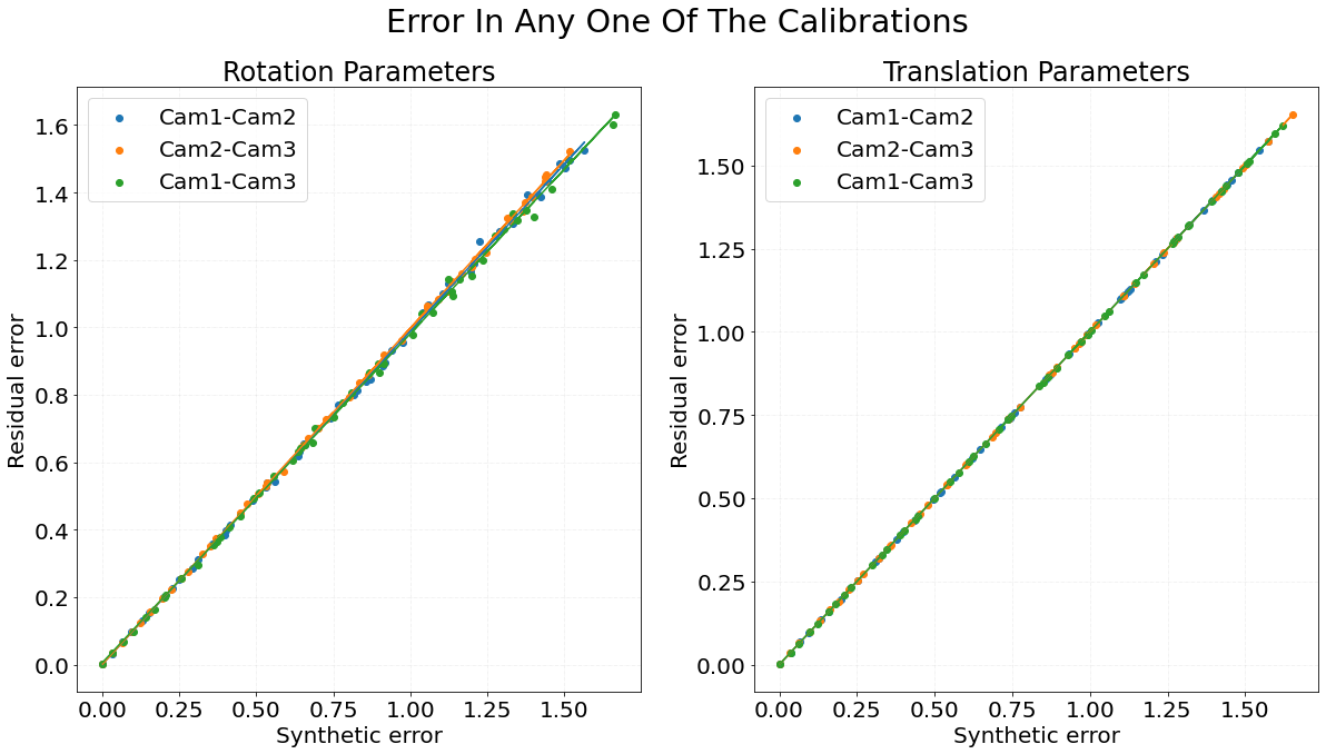
Graph 1 shows the residual error of a group of three sensors on the Y-axis while X-axis represents the random error added to each of the three calibrations. The color indicates the results for three experiments where the error was added only to the calibration corresponding to the respective color in the legend i.e. the other calibrations remain as original and only one of them gets the synthetic error added to it. The slope of the line fitted on points (rotation, translation) is (0.989, 0.999) for blue dots, (0.997, 0.999) for orange dots, (0.975, 1.000) for green dots.
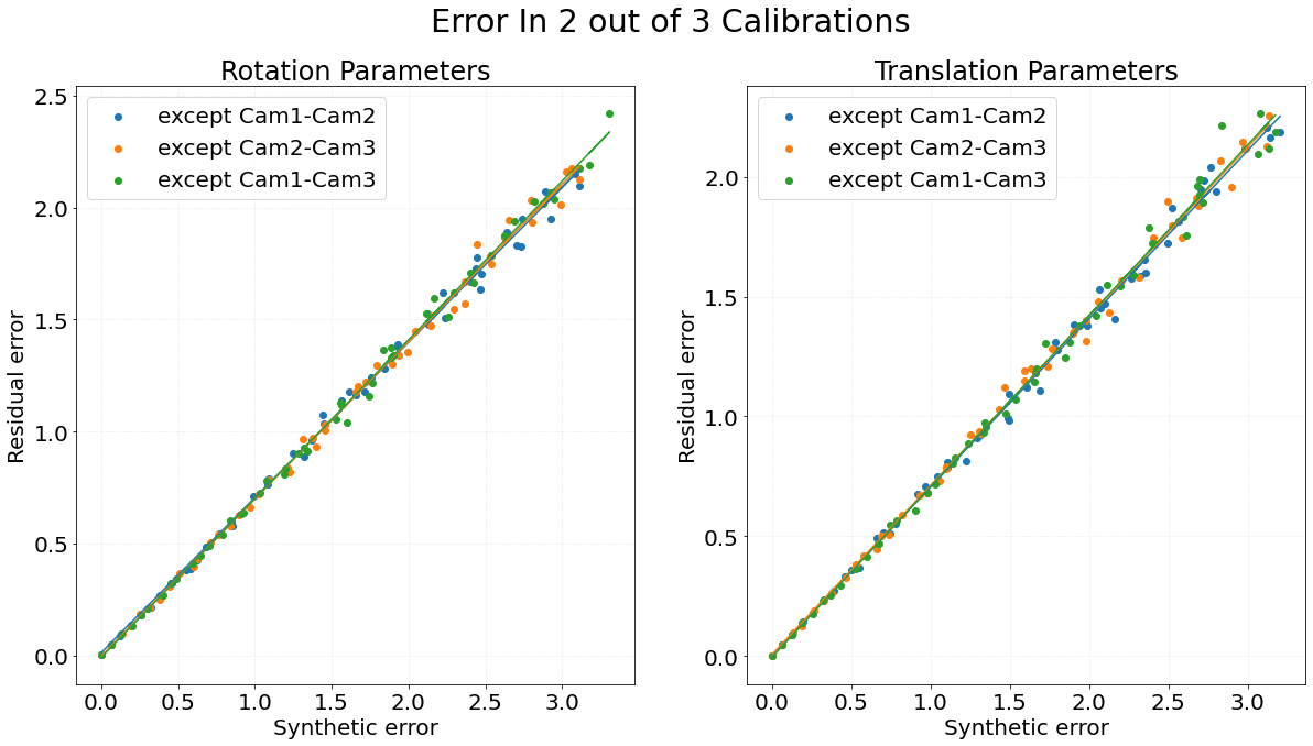
Graph 2 shows the residual error of a group of three sensors on the Y-axis while X-axis represents the random error added to any two calibrations. The color indicates the results for three experiments where the error was added only to two calibrations except the one corresponding to the respective color in the legend i.e. the calibration in the legend remains as original while the others get the synthetic error added to it. The slope of the line fitted on points (rotation, translation) is (0.692, 0.703) for blue dots, (0.702, 0.707) for orange dots, (0.709, 0.713) for green dots.
Graph 3 shows the residual error of a group of three sensors on the Y-axis while X-axis represents the random error added to all three calibrations. This experiment indicates the results of an experiment where the error was added to all three calibrations. The slope of the line fitted on points is 0.561 for rotation parameters and 0.575 for translation parameters. Additionally, we found that the individual error before optimisation can be estimated by dividing the constants 2.478 for rotation parameters and 1.966 for translational parameters from the residual error. These estimates are calculated from the simulated data and hold true only if the error is distributed uniformly.
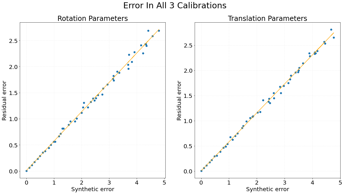
We can observe that increasing calibrations with synthetic error decreases the slope between residual error and synthetic error. Due to high correlation between individual calibrations and residual error, we can use residual error as a way to estimate the accuracy of individual calibration.
